Click here if you missed the previous parts of this article: part I
Factorial analysis: HVAC Thermal Energy Consumption vs Outside Temperature
Assumed the abovementioned simplification, we will now go on to identify the variables on which the consumption of thermal energy in an office, in a home, depends, starting from the fact that we wish to maintain a constant temperature inside. That is, to perform a factorial analysis.
Let’s go to revise which independent variables we can identify:
- Outside Temperature
- Days of the week and hours of the day we want to maintain the indoor temperature
- Relative humidity (depends partially on the temperature) Occupancy rate
- Thermal inertia of the building
- Heat gains due to solar radiation
- Ventilation, opening of windows
- Other thermal energy loads (lighting, computers, cooking)
If we focus on a specific building, it is possible that some of these variables may become a constant, such as the hours of operation in an office, the opening hours of a shop, or the lighting schedule. Others, such as the degree of occupancy, may be considered constant in an office, but not in a shopping centre or even in a house.
The next step will be to focus on the outside temperature as “the” variable, the main one, the only one, without forgetting the simplification we have granted ourselves when interpreting the results.
Now, going on with the imaginary building on which we are focusing our analysis, let us imagine that we are able to know on what date the heating was turned on and on what date the cooling was turned on for the last 10 years, assuming that the indoor setpoint temperature would be of 21-23ºC in winter and 24-26ºC in summer.
With this information, let’s analyse what the average temperature was on the three days prior to the start-up of the climate system in each of those 10 years. We would dare to expect a value around 15-18ºC of the outside temperature when the heating was switched on, which we will call the base heating temperature, and 18-21ºC when switching on the cooling, which we will call the base cooling temperature.
Thus, and with the limitations set out above, we end up stating that:
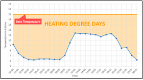
The consumption of thermal energy applied to heating is a function of the difference between the outside temperature and the value of the base heating temperature referred to above. We will call this difference Heating Degree-Days[3], and we will apostille it with the base temperature (15 to 18ºC) with which we have calculated these Heating Degree-Days. E.g.: HDD15
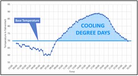
Repeating the same concept for summer, we will have that the energy consumption dedicated to cooling is a function of the Cooling Degree-Days, and we will also apostille it with the base temperature (18-21ºC) that we have used for its calculation. E.g.: CDD20
Linear regression line – Baseline
Let us now analyse the expression we have used “is a function of“. Let’s see what kind of function it is.
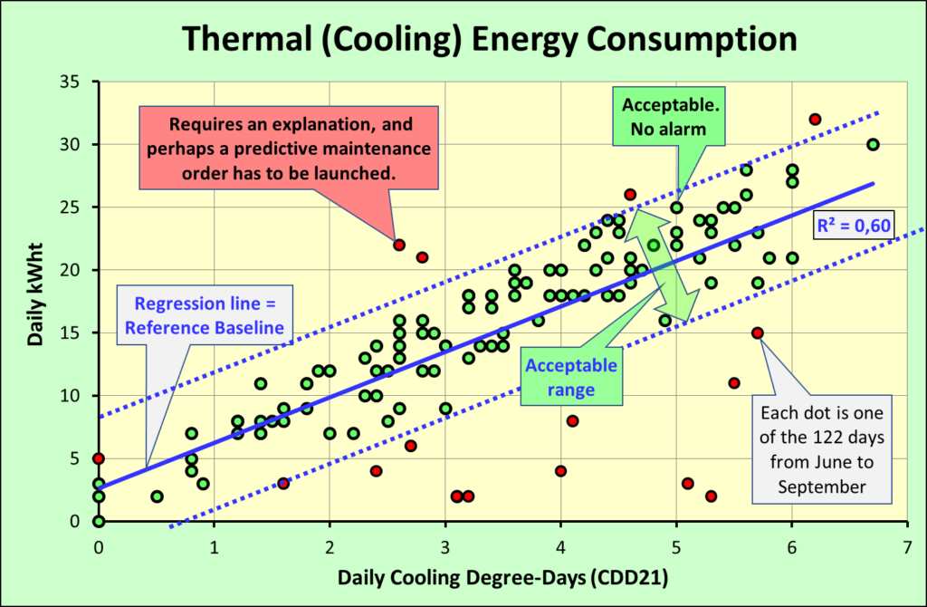
We will demonstrate this function with empirical data. Both variables (Thermal Energy and Outside Temperature) are monitored and displayed graphically. We can appreciate that the dependence is linear, and, if we have chosen the right base temperature for the calculation of the Degree-Days, this straight line crosses the origin of the coordinates of the graph. That is to say, for Degree-Days = zero, the consumption of thermal energy = zero, and rises proportionally to the Degree-Days, responding to the most elementary thermodynamic criteria.
It is now up to us to explain with which is the period of time we select to analyse this function.
Depending on the purpose at hand, we may use different time units. The two most relevant units will be those that represent a closed cycle of the outside temperature. That is: the day, and the year. The week can also be used, and the month too. But in this case, certain adjustments have to be made in the use of the month, since for the same number of monthly Degree-Days, a month of 30 days and a month of 31 days would really have different energy consumptions, and this would be against the rule.
But let’s go forward:
Conceptually, the Degree-Days value corresponds to the surface shown in the graphs below. The Degree-Days value for each day is obtained by integrating the Degrees-Day curve for each ∆ of time. So, what ∆t is taken in practice to carry out these calculations?
Nowadays, thanks to the ease with which sensorics and monitoring processes are made available to professionals, the data can be collected every minute and less without any difficulty. However, taking into account that the temperature, unlike wind, solar radiation or rainfall, has an evolution without significant discontinuities, and confirmed by our own experience in practical application, it is possible to work with hourly values without losing any representativeness, although for greater peace of mind, it can be done with quarter-hourly values. Time-slot values of less than 15 minutes do not make any sense in this case.
The regression and correlation analysis starts from a point cloud. One point for each day, or one for each year, etc. depending on what we have chosen as the unit depending on the purpose we are pursuing. And from that point cloud we obtain the linear regression line, directly from Excel. Associated with it we will have the R2 value, which informs us about the reliability of this supposed relationship between Energy Consumption and Degree-Days.
Let’s continue our exercise. If we are talking about Degrees-Day, which days of the year will be chosen to introduce their data in the correlation analysis between Energy Consumption and Degree-Days?
It is logical to imagine that on days with very low Degree-Days values, the influence of these few Degree-Days on consumption may be masked by other variables that we have assumed to be constant, but which in reality are not so constant (occupancy, ventilation, etc.), so it would be better to disregard them. Which are the days with few Degree-Days? Very easy: those at the beginning and at the end of the cold season and those at the beginning and at the end of the warm season.
Going a little deeper into these concepts and always based on experience, a consensus has been reached, and in Mediterranean climatology it is applied that:
- Period of correlation analysis of the cold season: November-March
- Period of correlation analysis of the warm season: June-September.
These correlation lines are the so-called Baselines within the IPMVP[4] protocol and the M&V procedures derived from it.
But to calculate this Baseline, it is necessary to have a point cloud. And the following question is: What minimum number of points (days) are needed to obtain a regression line sufficiently representative of the building in question? Five years would be ideal, three is desirable, and if you only have one, then you have to make do.
That’s taking into account that one day is one point. But be careful, do all the days have useful data to this purpose? Does any day have a valid relation of consumption vs Degree-Days? To know the response, we return to the variables, and we see that one of them is the timetable. Well, in an office building, days with the same timetable are usually from Monday to Thursday. On Friday, work time usually ends at midday, and in the afternoon the office is closed, or even if it is not closed, another variable that we have considered as fixed for simplicity, which is occupancy, is not fulfilled, because although the office may remain open, the number of users may be much lower. And there is another variable that further limits the range of eligible days. Monday must be discarded, as it drags the thermal inertia of the building because it has not been air-conditioned the day before. Then, out of 7 days, we are left with three, or in other words, out of the 151 days of the cold season analysis period (Nov-Mar), we are left with only 64 points to deduce the HDD regression line, and out of the 122 days of the warm season (Jun-Sep), we are left with only 52 points to deduce the CDD regression line.
For each type of building, the selection of eligible days for the correlation analysis will basically depend on its hours of operation. At the residential level, in dwellings, it will depend on the schedule of the users, their weekend habits, etc.
Beyond this simple and useful method of analysis, more complex algorithms can be developed, in which the factorial analysis goes on to consider other variables as independent. A clear example would be the number of visitors to a museum, given that it can vary considerably. But this goes beyond the aims of our article.
References
3. Degree-Days measures how cold or warm a location is. A Degree-Day compares the current outdoor temperature recorded for a location to a base temperature. The more extreme the outside temperature, the higher the number of degree days. A high number of degree days generally results in higher levels of energy use for space sir conditioning.
4.The International Performance Measurement and Verification Protocol (IPMVP®) defines standard terms and suggests best practices for quantifying the results of energy efficiency investments through Measurement & Verification (M&V) protocols. The IPMVP was developed by a coalition of international organizations starting in 1994-1995.
Written by Antoni Quintana, from COMSA